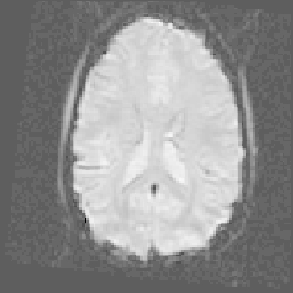
Functional Magnetic Resonance Imaging (fMRI)

This page is only an overview of the main concepts, and also covers the standard processing and analysis methods used in fMRI studies. Consider reading Huettel et al. (2004) for a more thorough introduction.

Nuclear particles, such as protons and neutrons, have a magnetic property called spin, which behaves much like an ordinary dipole-magnet. Usually, the focus of interest is on hydrogen nuclei, because of their abundance in all tissue types and relatively simple spin behavior. The behavior of the nuclear spin of heavier atoms is more complicated, since there are internal interactions between the individual particles. Fundamentally, all MR-imaging is based on the interaction between the imaged tissue, externally applied magnetic fields and carefully synchronized radio frequency pulses.

Under a very strong and uniform magnetic field, the spins try to align parallel to the field either in the same or opposite directions. More precisely, the spins precess around those directions in a minimum energy state. Although the precession is not coherent, all the spins have a characteristic resonance frequency, proportional to the strength of the magnetic field. When a radio pulse in the resonance frequency is emitted, the spins absorb the energy and are forced into coherent precession. After the pulse, the absorbed energy decays in a relaxation process. The process is actually quite complex, for example, due to possible internal interactions in the tissue. However, signals measuring the decay of energy make the imaging possible, and adjusting the properties and timing of the radio pulses produces signals related to different aspects of the relaxation process.

To produce a volumetric (3-dimensional) image, the behavior of the spins is controlled more precisely with two gradient magnetic fields, which are perpendicular to each other. The first is applied in the same direction as the uniform magnetic field, causing the total strength of the field to change slightly along that direction. This makes the resonance frequency of the spins also different along its axis. The other gradient field is similar, but turned on and off repeatedly. As the spins precess faster during the application of the field, the spins along its axis accumulate different phases. The gradient magnetic fields allow focusing on a planar slice, which is defined by the axes of frequency-phase space. Carefully synchronizing the radio pulses with the fields produces signals originating from different parts of the slice. Additionally, the thickness of the slice can be controlled with the bandwidth of the radio pulses.

Using standard signal processing techniques, the measurements can be turned into an image of the focused slice. The full volume is produced by scanning several adjacent slices, one after the other. The image voxels contain a kind of density measure based on the scanning parameters and the properties of the tissue. For example, with certain parameters the image is directly related to the proton density of the tissue.

The scanning is actually very slow since the relaxation process, and adjusting the magnetic fields, requires a certain amount of time. Producing high resolution images can take several minutes. Naturally, the quality of the images is strongly affected by inhomogeneities in the magnetic fields, the internal magnetic interactions and electromagnetic interference from the environment.

Since MRI is virtually noninvasive and is able to produce high quality images, it has quickly become very popular in structural imaging. These properties are crucial also in functional imaging, but the measures used in structural MRI, such as the proton density, are not directly related to neuronal activation. Coincidentally, the scanning parameters can be tuned so that the resulting images provide a measure related to the oxygenation level in the tissue. The measure is based on the differing magnetic properties of oxygenated and deoxygenated hemoglobin molecules, as further explained in the next section. The idea in functional MRI is to record a sequence of such images at different time points to allow the local changes in oxygenation level to be analyzed.

Problems arise from the long duration of the scanning. Scanning intervals of several minutes would not allow accurate analysis of the activity in the brain. Additionally, movement of the head and other physiological changes during the long exposures would distort the images. Fortunately, the scanning parameters, mainly the timing of the radio pulses, can be adjusted to allow much faster scanning. However, the spatial resolution suffers greatly from such adjustments. For example, the relaxation process is not allowed to fully complete, resulting in much weaker signals. Therefore, the setup used in fMRI is a careful compromise between fast scanning and high resolution images. Current fMRI scanners are able to produce full head volumes with a time interval of a few seconds, but the spatial resolution is only a fraction of that used in structural imaging.

Measuring Hemodynamic Responses to Stimuli

The detection of changes due to neuronal activation in fMRI is based on the differing magnetic properties of oxygenated (diamagnetic) and deoxygenated (paramagnetic) hemoglobin molecules. Neuronal activation results in a localized change of blood flow and oxygenation levels, which can be measured using suitable scanning parameters. This produces a measure called blood oxygenation level dependent (BOLD) signal (c.f., Ogawa et al., 1992). These vascular or hemodynamic changes are related to the electrical activity of neurons in a complex and delayed way. Local changes in the level of oxygenation reveal the active areas, but it is not possible to completely recover the electrical processes from the vascular ones. The hemodynamic changes are hard to model, but as their nature is somewhat slow and smoothly varying, a Gaussian model is often used. Some newer models of the hemodynamic response function are actually based on measurements from the real brain.

Usually, fMRI studies use a controlled stimulus, like visual patterns or audible beeps, designed to test a specific hypothesis. The simplest way of doing this is to repeat the stimulus several times, with resting periods in between, and scan the fMRI sequence during the whole time. Such experiments should reveal areas of the brain that are always active during the stimulation and inactive during the resting. Sometimes the subject can even be asked to perform a relatively simple mental or motor task during the scanning. Naturally, such tasks should not be allowed to result in head movement.

One example of an fMRI study is shown in Figure 1(a). The low resolution and the scanning parameters, optimized for BOLD, make the contrast between different tissue types very poor. Additionally, the fast scanning and low signal-to-noise ratio of the BOLD signal make the image very noisy. Therefore, a high resolution structural MRI is often scanned separately to aid in locating the activation during analysis by super-positioning. The bright areas in the images do not necessarily correspond to the active ones. Careful analysis of the whole sequence is required to detect the activation patterns.

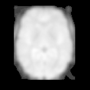
**Figure 1:** Examples of functional magnetic resonance images. (a) A scanned slice without processing and (b) after the standard preprocessing has been applied. Note that the images do not show a direct measure of activation.
(a)	(b)

Standard Preprocessing of Images

In addition to the low signal-to-noise ratio and additive noise, seen in Figure 1(a), the fMRI measurements are contaminated with artifacts, such as head movement and physiological vascular changes. Thus, the detection and analysis of interesting phenomena is very difficult. To overcome these difficulties, the images need to be preprocessed (c.f., Worsley and Friston, 1995, SPM, 1999). Figure 1(b) shows an example slice after preprocessing. The level of noise is clearly reduced and the values are much more continuous. Also, the excess area outside the brain has been removed, and is shown in black. The usual steps of the preprocessing include:

Retiming the slices to account for the fact that each slice was scanned at a slightly different time. Since the scanning is not instantaneous this kind of temporal smoothing improves the continuity of the measurements.
Realigning the slices to reduce head movement related artifacts. This makes the voxels of different time points match spatially and removes some of the empty area surrounding the head in the images.
Smoothing or low-pass filtering to reduce high frequency noise and to increase local voxel correlations. This increases the signal-to-noise ratio of the hemodynamic effect and makes detection of interesting phenomena easier.
Normalizing the volumes into a standard coordinate system. This allows comparing different scans and identifying known locations.

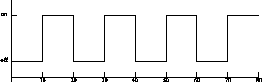
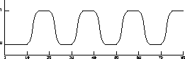
The normalization step is not required for analysis, but is often done to match the functional volumes to the structural ones. Additionally, the normalization makes comparisons between different subjects easier. In practice, this may somewhat distort the brain in the images and individual differences may still remain quite big, so that caution needs to be taken when drawing inter-subject conclusions.

Standard Analysis of fMRI Sequences

The standard way of analyzing an fMRI sequence is to use statistical parametric mapping (SPM), which is based on a general linear model (GLM) (c.f., Worsley and Friston, 1995). Essentially, the analysis reveals the areas of the brain that most probably fit a given hypothesis, which is presented as a reference time-course.

The reference time-course can be approximated using the stimulation pattern and a model of the hemodynamic response. An example of such a reference time-course is shown in Figure 2. The depicted pattern is a very simple case of repeated on-off type of stimulus. The stimulation time-course is then convolved with the model of the hemodynamic response, assumed Gaussian in the illustration.

**Figure 2:** Illustration of an ideal stimulus. (a) An ideal stimulation time-course comprising of rest and activation periods. (b) The corresponding ideal reference time-course convolved with the hemodynamic response. In reality the detected time-course varies significantly.
(a)	(b)

The analysis can be considered in two steps. First, the reference time-course is compared to the time-course of each voxel in the fMRI sequence statistically. This produces an image of the probability to fit the given time-course, where the voxels with the highest probabilities are considered to be active. However, the probability image is very noisy and the second step is to segment it into the inactive and active areas. The segmentation is made robust by using a statistical model for the noise, usually assumed Gaussian. The difficulty with this approach is to define a threshold for the probability of activation that produces an accurate segmentation. Choosing a too high value value easily leads to discontinuous or too small areas. On the other hand, a small value may produce big areas that do not accurately locate the activation of interest.

After the spatial activation patterns have been formed, the true activation time-course of each area is formed by taking the mean sequence of all the voxels in the area. Again, if the segmentation is poor, for example, due to an incorrect threshold value, the time-courses are not generated accurately.

There are big problems with such analysis. The accuracy is limited by the ability to approximate the parameters needed for the statistical fitting. Also, small changes to the parameters can change the results severely. Additionally, the stimulation setup has to be simple enough to allow predicting the responses, and forming the reference time-courses, in the first place. Therefore, detecting previously unknown phenomena is extremely hard or close to impossible. These are some of the reasons why current research focuses on more data-driven and adaptive methods, like independent component analysis (ICA).

TODO: Explanation of relation to ni...