Simulation and experimental results

First, we investigated the robustness of the contrast functions. We generated four artificial source signals, two of which were sub-Gaussian, and two were super-Gaussian. The source signals were mixed using several different random matrices, whose elements were drawn from a standardized Gaussian distribution. To test the robustness of our algorithms, four outliers whose values were $\pm 10$ were added in random locations. The fixed-point algorithm for sphered data was used with the three different contrast functions in eq. (14-16), and symmetric orthogonalization. Since the robust estimation of the covariance matrix is a classical problem independent of the robustness of our contrast functions, we used in this simulation a hypothetical robust estimator of covariance, which was simulated by estimating the covariance matrix from the original data without outliers. In all the runs, it was observed that the estimates based on kurtosis (16) were essentially worse than the others, and estimates using G₂ in (15) were slightly better than those using G₁ in (14). These results confirm the theoretical predictions on robustness in Section 3.

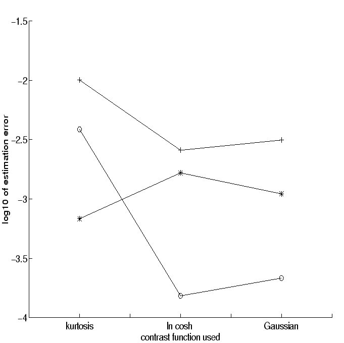
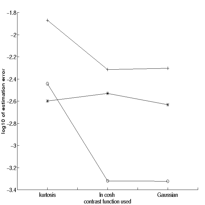
To investigate the asymptotic variance, i.e., efficiency, of the estimators, we performed simulations in which the 3 different contrast functions were used to estimate one independent component from a mixture of 4 identically distributed independent components. We also used three different distributions of the independent components: uniform, double exponential (or Laplace), and the distribution of the third power of a Gaussian variable. The asymptotic mean absolute deviations (which is a robustified measure of error) between the components of the obtained vectors and the correct solutions were estimated and averaged over 1000 runs for each combination of non-linearity and distribution of independent component. The results in the basic, noiseless case are depicted in Fig. 1. As one can see, the estimates using kurtosis were essentially worse for super-Gaussian independent components. Especially the strongly super-Gaussian independent component (cube of Gaussian) was estimated considerably worse using kurtosis. Only for the sub-Gaussian independent component, kurtosis was better than the other contrast functions. There was no clear difference between the performances of the contrast functions G₁ and G₂. Next, the experiments were repeated with added Gaussian noise whose energy was 10% of the energy of the independent components. The results are shown in Fig. 2. This time, kurtosis did not perform better even in the case of the sub-Gaussian density. The robust contrast functions seem to be somewhat robust against Gaussian noise as well.

We also studied the speed of convergence of the fixed-point algorithms. Four independent components of different distributions (two subgaussian and two supergaussian) were artificially generated, and the symmetric version of the fixed-point algorithm for sphered data was used. The data consisted of 1000 points, and the whole data was used at every iteration. We observed that for all three contrast functions, only three iterations were necessary, on the average, to achieve the maximum accuracy allowed by the data. This illustrates the fast convergence of the fixed-point algorithm. In fact, a comparison of our algorithm with other algorithms was performed in [13], showing that the fixed-point algorithm gives approximately the same statistical efficiency as other algorithms, but with a fraction of the computational cost.

Experiments on different kinds of real life data have also been performed using the contrast functions and algorithms introduced above. These applications include artifact cancellation in EEG and MEG [36,37], decomposition of evoked fields in MEG [38], and feature extraction of image data [35,25]. These experiments further validate the ICA methods introduced in this paper. A $\mbox{Matlab}^{TM}$ implementation of the fixed-algorithm is available on the World Wide Web free of charge [10].

  

Figure 1: Finite-sample estimation errors plotted for different contrast functions and distributions of the independent components, in the noiseless case. Asterisk: uniform distribution. Plus sign: Double exponential. Circle: cube of Gaussian.

  

Figure 2: The noisy case. Finite-sample estimation errors plotted for different contrast functions and distributions of the independent components. Asterisk: uniform distribution. Plus sign: Double exponential. Circle: cube of Gaussian.