Motivation

Imagine that you are in a room where two people are speaking simultaneously. You have two microphones, which you hold in different locations. The microphones give you two recorded time signals, which we could denote by x₁(t) and x₂(t), with x₁ and x₂ the amplitudes, and t the time index. Each of these recorded signals is a weighted sum of the speech signals emitted by the two speakers, which we denote by s₁(t) and s₂(t). We could express this as a linear equation:
 $$\begin{align} x_1(t)=a_{11} s_1 + a_{12} s_2\\ x_2(t)=a_{21} s_1 + a_{22} s_2 \end{align}$$
where a₁₁,a₁₂,a₂₁, and a₂₂ are some parameters that depend on the distances of the microphones from the speakers. It would be very useful if you could now estimate the two original speech signals s₁(t) and s₂(t), using only the recorded signals x₁(t) and x₂(t). This is called the cocktail-party problem. For the time being, we omit any time delays or other extra factors from our simplified mixing model.

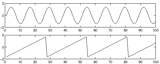
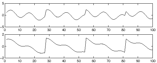
As an illustration, consider the waveforms in Fig. 1 and Fig. 2. These are, of course, not realistic speech signals, but suffice for this illustration. The original speech signals could look something like those in Fig. 1 and the mixed signals could look like those in Fig. 2. The problem is to recover the data in Fig. 1 using only the data in Fig. 2.

  

Figure 1: The original signals.

  

Figure 2: The observed mixtures of the source signals in Fig. 1.

  

Figure 3: The estimates of the original source signals, estimated using only the observed signals in Fig. 2. The original signals were very accurately estimated, up to multiplicative signs.

Actually, if we knew the parameters a_ij, we could solve the linear equation in (1) by classical methods. The point is, however, that if you don't know the a_ij, the problem is considerably more difficult.

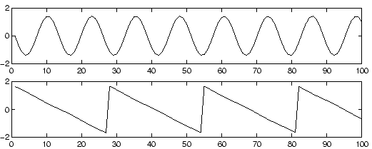
One approach to solving this problem would be to use some information on the statistical properties of the signals s_i(t) to estimate the a_ii. Actually, and perhaps surprisingly, it turns out that it is enough to assume that s₁(t) and s₂(t), at each time instant t, are statistically independent. This is not an unrealistic assumption in many cases, and it need not be exactly true in practice. The recently developed technique of Independent Component Analysis, or ICA, can be used to estimate the a_ij based on the information of their independence, which allows us to separate the two original source signals s₁(t) and s₂(t) from their mixtures x₁(t) and x₂(t). Fig. 3 gives the two signals estimated by the ICA method. As can be seen, these are very close to the original source signals (their signs are reversed, but this has no significance.)

Independent component analysis was originally developed to deal with problems that are closely related to the cocktail-party problem. Since the recent increase of interest in ICA, it has become clear that this principle has a lot of other interesting applications as well.

Consider, for example, electrical recordings of brain activity as given by an electroencephalogram (EEG). The EEG data consists of recordings of electrical potentials in many different locations on the scalp. These potentials are presumably generated by mixing some underlying components of brain activity. This situation is quite similar to the cocktail-party problem: we would like to find the original components of brain activity, but we can only observe mixtures of the components. ICA can reveal interesting information on brain activity by giving access to its independent components.

Another, very different application of ICA is on feature extraction. A fundamental problem in digital signal processing is to find suitable representations for image, audio or other kind of data for tasks like compression and denoising. Data representations are often based on (discrete) linear transformations. Standard linear transformations widely used in image processing are the Fourier, Haar, cosine transforms etc. Each of them has its own favorable properties [15].

It would be most useful to estimate the linear transformation from the data itself, in which case the transform could be ideally adapted to the kind of data that is being processed. Figure 4 shows the basis functions obtained by ICA from patches of natural images. Each image window in the set of training images would be a superposition of these windows so that the coefficient in the superposition are independent. Feature extraction by ICA will be explained in more detail later on.

  

Figure: Basis functions in ICA of natural images. The input window size was $16 \times 16$ pixels. These basis functions can be considered as the independent features of images.

All of the applications described above can actually be formulated in a unified mathematical framework, that of ICA. This is a very general-purpose method of signal processing and data analysis.

In this review, we cover the definition and underlying principles of ICA in Sections 2 and 3. Then, starting from Section 4, the ICA problem is solved on the basis of minimizing or maximizing certain conrast functions; this transforms the ICA problem to a numerical optimization problem. Many contrast functions are given and the relations between them are clarified. Section 5 covers a useful preprocessing that greatly helps solving the ICA problem, and Section 6 reviews one of the most efficient practical learning rules for solving the problem, the FastICA algorithm. Then, in Section 7, typical applications of ICA are covered: removing artefacts from brain signal recordings, finding hidden factors in financial time series, and reducing noise in natural images. Section 8 concludes the text.