Illustration of ICA

To illustrate the ICA model in statistical terms, consider two independent components that have the following uniform distributions:

$$p(s_i)= \begin{cases}\frac{1}{2\sqrt{3}}& \text{if } \vert s_i\vert\leq\sqrt{3}\\ 0 & \text{otherwise} \end{cases}$$ (5)

The range of values for this uniform distribution were chosen so as to make the mean zero and the variance equal to one, as was agreed in the previous Section. The joint density of s₁ and s₂ is then uniform on a square. This follows from the basic definition that the joint density of two independent variables is just the product of their marginal densities (see Eq. 10): we need to simply compute the product. 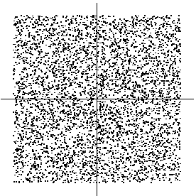The joint density is illustrated in Figure 5 by showing data points randomly drawn from this distribution.

  

Figure 5: The joint distribution of the independent components s₁and s₂ with uniform distributions. Horizontal axis: s₁, vertical axis: s₂.

  

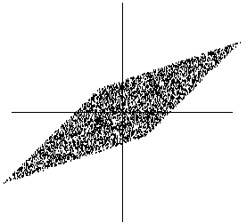
Figure 6: The joint distribution of the observed mixtures x₁ and x₂. Horizontal axis: x₁, vertical axis: x₂.

Now let as mix these two independent components. Let us take the following mixing matrix:

$${\bf A}_0=\begin{pmatrix}2 & 3\\ 2 & 1 \end{pmatrix}$$ (6)

This gives us two mixed variables, x₁ and x₂. It is easily computed that the mixed data has a uniform distribution on a parallelogram, as shown in Figure 6. Note that the random variables x₁ and x₂ are not independent any more; an easy way to see this is to consider, whether it is possible to predict the value of one of them, say x₂, from the value of the other. Clearly if x₁ attains one of its maximum or minimum values, then this completely determines the value of x₂. They are therefore not independent. (For variables s₁ and s₂ the situation is different: from Fig. 5 it can be seen that knowing the value of s₁ does not in any way help in guessing the value of s₂.)

The problem of estimating the data model of ICA is now to estimate the mixing matrix ${\bf A}_0$ using only information contained in the mixtures x₁ and x₂. Actually, you can see from Figure 6 an intuitive way of estimating ${\bf A}$: The edges of the parallelogram are in the directions of the columns of ${\bf A}$. This means that we could, in principle, estimate the ICA model by first estimating the joint density of x₁ and x₂, and then locating the edges. So, the problem seems to have a solution.

In reality, however, this would be a very poor method because it only works with variables that have exactly uniform distributions. Moreover, it would be computationally quite complicated. What we need is a method that works for any distributions of the independent components, and works fast and reliably.

Next we shall consider the exact definition of independence before starting to develop methods for estimation of the ICA model.