Principal component analysis

Principal Component Analysis, or PCA (see [77,87]), is widely used in signal processing, statistics, and neural computing. In some application areas, this is also called the (discrete) Karhunen-Loève transform, or the Hotelling transform.

The basic idea in PCA is to find the components s₁,s₂,...,s_n so that they explain the maximum amount of variance possible by nlinearly transformed components. PCA can be defined in an intuitive way using a recursive formulation. Define the direction of the first principal component, say ${\bf w}_1$, by

$${\bf w}_1=\arg\max_{\Vert{\bf w}\Vert=1} E\{({\bf w}^T{\bf x})^2\}$$ (3)

where ${\bf w}_1$ is of the same dimension m as the random data vector ${\bf x}$. (All the vectors in this paper are column vectors). Thus the first principal component is the projection on the direction in which the variance of the projection is maximized. Having determined the first k-1 principal components, the k-th principal component is determined as the principal component of the residual:

$${\bf w}_{k}=\arg\max_{\Vert{\bf w}\Vert=1} E\{[{\bf w}^T({\bf x}-\sum_{i=1}^{k-1}{\bf w}_i{\bf w}_i^T{\bf x})]^2\}$$ (4)

The principal components are then given by $s_i={\bf w}_i^T{\bf x}$. In practice, the computation of the ${\bf w}_i$ can be simply accomplished using the (sample) covariance matrix $E\{{\bf x}{\bf x}^T\}={\bf C}$. The ${\bf w}_i$ are the eigenvectors of ${\bf C}$ that correspond to the n largest eigenvalues of ${\bf C}$.

The basic goal in PCA is to reduce the dimension of the data. Thus one usually chooses n<<m. Indeed, it can be proven that the representation given by PCA is an optimal linear dimension reduction technique in the mean-square sense [77]. Such a reduction in dimension has important benefits. First, the computational overhead of the subsequent processing stages is reduced. Second, noise may be reduced, as the data not contained in the n first components may be mostly due to noise. Third, a projection into a subspace of a very low dimension, for example two, is useful for visualizing the data. Note that often it is not necessary to use the n principal components themselves, since any other orthonormal basis of the subspace spanned by the principal components (called the PCA subspace) has the same data compression or denoising capabilities.

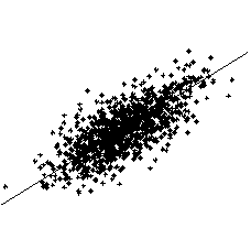
A simple illustration of PCA is found in Fig. 1, in which the first principal component of a two-dimensional data set is shown.

  

Figure 1: Principal component analysis of a two-dimensional data cloud. The line shown is the direction of the first principal component, which gives an optimal (in the mean-square sense) linear reduction of dimension from 2 to 1 dimensions.