


Next: Fixed-point algorithm for several
Up: Fixed-point algorithms for ICA
Previous: Introduction
Fixed-point algorithm for one unit
To begin with, we shall derive the fixed-point algorithm for one unit,
with sphered data.
First note that the maxima of
 are obtained at certain optima
of
are obtained at certain optima
of
 .
According to the Kuhn-Tucker conditions [29], the optima
of
under
the constraint
.
According to the Kuhn-Tucker conditions [29], the optima
of
under
the constraint
 are obtained at points
where
are obtained at points
where
 |
(17) |
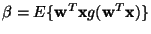
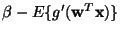
where  is a constant that can be easily evaluated to give
 ,
where
,
where  is the value of
  at the optimum. Let us try to solve this equation by
Newton's method. Denoting the function on the left-hand side of
(17) by F, we obtain its Jacobian matrix
at the optimum. Let us try to solve this equation by
Newton's method. Denoting the function on the left-hand side of
(17) by F, we obtain its Jacobian matrix
 as
as
 |
(18) |
To simplify the inversion of this matrix, we decide to approximate the first
term in (18). Since the data is sphered, a reasonable
approximation seems to be
 .
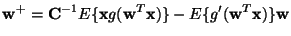
Thus the Jacobian matrix becomes
diagonal, and can easily be inverted. We also approximate using the current value of
instead of .
Thus we obtain the
following approximative Newton iteration:
.
Thus the Jacobian matrix becomes
diagonal, and can easily be inverted. We also approximate using the current value of
instead of .
Thus we obtain the
following approximative Newton iteration:
![\begin{displaymath}
\begin{split}
{\bf w}^+={\bf w}-[E\{{\bf x}g({\bf w}^T{\bf x...
...-\beta] \\
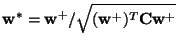
{\bf w}^*={\bf w}^+/\Vert{\bf w}^+\Vert
\end{split}\end{displaymath}](img69.gif) |
(19) |
where  denotes the new value of ,
 ,
and the normalization has been added to improve the stability.
This algorithm can be further simplified by multiplying both sides of the
first equation in (19) by
,
and the normalization has been added to improve the stability.
This algorithm can be further simplified by multiplying both sides of the
first equation in (19) by
 .
This
gives the following fixed-point algorithm
.
This
gives the following fixed-point algorithm
 |
(20) |
which was introduced in [17] using a more heuristic
derivation. An earlier version (for kurtosis only) was derived as a
fixed-point iteration of a neural learning rule in
[23], which is where its name comes from. We retain
this name for the algorithm,
although in the light of the above derivation, it is rather a Newton
method than a fixed-point iteration.
Due to the approximations used in the derivation of the fixed-point
algorithm, one may wonder if it really converges to the right
points. First of all, since only the Jacobian
matrix is approximated, any convergence point of the algorithm must be
a solution of the Kuhn-Tucker condition in (17). In
Appendix A it is further
proven that the algorithm does converge to the right extrema
(those corresponding to maxima of the contrast function),
under the assumption of the ICA data model. Moreover, it is proven that the
convergence is quadratic, as usual with Newton methods. In fact, if
the densities of the si are symmetric, the convergence is even
cubic. The convergence proven in the Appendix is local. However, in
the special case where
kurtosis is used as a contrast function, i.e., if G(u)=u4, the
convergence is proven globally.
The above derivation also enables a useful modification of the fixed-point
algorithm. It is well-known that the convergence of the Newton method
may be rather uncertain. To ameliorate this, one may add a step size
in (19), obtaining the stabilized fixed-point algorithm
![\begin{displaymath}
\boxed{
\begin{split}
{\bf w}^+={\bf w}-\mu[E\{{\bf x}g({\bf...
...\beta] \\
{\bf w}^*={\bf w}^+/\Vert{\bf w}^+\Vert
\end{split}}\end{displaymath}](img74.gif) |
(21) |
where
as above, and  is a step size parameter that may
change with the iteration count. Taking a
that is much smaller
than unity (say, 0.1 or 0.01), the algorithm (21) converges
with much more certainty. In
particular, it is often a good strategy to start with
is a step size parameter that may
change with the iteration count. Taking a
that is much smaller
than unity (say, 0.1 or 0.01), the algorithm (21) converges
with much more certainty. In
particular, it is often a good strategy to start with  ,
in
which case the algorithm is equivalent to the original fixed-point
algorithm in (20). If convergence seems problematic,
may
then be decreased gradually until convergence is satisfactory.
Note that we thus have a continuum between a Newton optimization
method, corresponding to ,
and a gradient descent method,
corresponding to a very small .
,
in
which case the algorithm is equivalent to the original fixed-point
algorithm in (20). If convergence seems problematic,
may
then be decreased gradually until convergence is satisfactory.
Note that we thus have a continuum between a Newton optimization
method, corresponding to ,
and a gradient descent method,
corresponding to a very small .
The fixed-point algorithms may also be simply used for the original,
that is, not sphered data. Transforming the data back to the
non-sphered variables, one sees easily that the following modification
of the algorithm (20) works for non-sphered data:
 |
|
|
|
 |
|
|
(22) |
where
 is the covariance matrix of the data. The
stabilized version, algorithm (21), can also be modified as follows
to work with non-sphered data:
is the covariance matrix of the data. The
stabilized version, algorithm (21), can also be modified as follows
to work with non-sphered data:
![$\displaystyle {\bf w}^+={\bf w}-\mu[{\bf C}^{-1}E\{{\bf x}g({\bf w}^T{\bf x})\}-\beta{\bf w}]/[E\{g'({\bf w}^T{\bf x})\}-\beta]$](img80.gif) |
|
|
|
|
|
|
(23) |
Using these two algorithms, one obtains directly an independent
component as the linear combination
 ,
where
,
where  need not be
sphered (prewhitened).
These modifications presuppose, of
course, that the covariance matrix is not singular. If it is singular
or near-singular, the dimension of the data must be reduced, for
example with PCA [7,28].
need not be
sphered (prewhitened).
These modifications presuppose, of
course, that the covariance matrix is not singular. If it is singular
or near-singular, the dimension of the data must be reduced, for
example with PCA [7,28].
In practice, the expectations in the fixed-point algorithms must be
replaced by their estimates. The natural estimates are of course the
corresponding sample means. Ideally, all the data available should
be used, but this is sometimes not a good idea because the computations
may become too demanding. Then the averages can be estimated using a
smaller sample, whose size may have a considerable effect on the
accuracy of the final estimates.
The sample points should be chosen separately at every iteration. If
the convergence is not satisfactory, one may then increase the sample
size. A reduction of the step size
in the stabilized version has
a similar effect, as is well-known in stochastic approximation methods
[24,28].
Next: Fixed-point algorithm for several
Up: Fixed-point algorithms for ICA
Previous: Introduction
Aapo Hyvarinen
1999-04-23