SOM implementation in SOM Toolbox

On this page, the structure of SOM and the SOM algorithm are described.

The indented paragraphs give further details of the implementation in SOM Toolbox.

In SOM Toolbox, all information regarding a SOM is gathered in a map struct. This struct has a number of fields, including the map codebook, map topology, component names and training history. There are also other structs, for example topology and training structs.

Structure of SOM

Map grid

A SOM is formed of neurons located on a regular, usually 1- or 2-dimensional grid. Also higher dimensional grids are possible, but they are not generally used since their visualization is much more problematic.

SOM Toolbox supports map grids of any dimension, although visualization is only supported for 1- and 2-dimensional maps. The map grid size is specified in the msize field of topology struct, which in turn is the topol field of the map struct, ie. the map grid specification of a map struct named sMap is sMap.topol.msize.

The neurons are connected to adjacent neurons by a neighborhood relation dictating the structure of the map. In the 2-dimensional case the neurons of the map can be arranged either on a rectangular or a hexagonal lattice, see Figure 1. If the sides of the map are connected to each other, the global shape of the map becomes a cylinder or a toroid, see figure Figure 2.

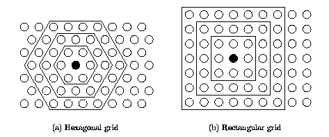Figure 1: Neighborhoods (size 1, 2 and 3) of the unit marked with black dot: (a) hexagonal lattice, (b) rectangular lattice.

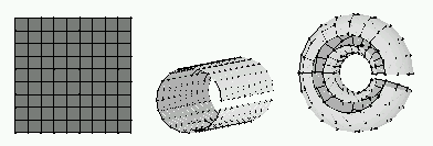Figure 2: Different map shapes: sheet on the left, cylinder in the center and toroid on the right. In the two latter, the connections across the gaps exist. They just have not been drawn.

SOM Toolbox supports both hexagonal and rectangular lattices and cylinder and toroid shapes. They are specified in the lattice and shape fields of the topology struct.

Prototypes

Each neuron i of the SOM has an associated d-dimensional prototype (aka weight, reference, codebook or model) vector m_i = [m_i1 m_i2 ... m_id], where d is equal to the dimension of the input vectors.

The prototype vectors of the map are in the codebook matrix of the map struct. The rows of the matrix sMap.codebook(i,:) are the prototype vectors and the columns sMap.codebook(:,i) are the variables (aka components). The map struct also has fields for names of the variables sMap.comp_names, normalization operations associated with each of the variables sMap.comp_norm as well as labels associated with each of the neurons sMap.labels.

Each neuron has actually two positions: one in the input space -- the prototype vector -- and another in the output space -- on the map grid. Thus, SOM is a vector projection method defining a nonlinear projection from the input space to a lower-dimensional output space. On the other hand, during the training the prototype vectors move so that they follow the probability density of the input data. Thus, SOM is also a vector quantization algorithm. Simplified, SOM is nothing more than an algorithm that combines these two tasks: vector quantization and projection.

Neighborhood function

Immediate neighbors, the neurons that are adjacent, belong to the 1-neighborhood N_i1 of the neuron i. Neighborhoods of different sizes in rectangular and hexagonal lattices are illustrated in Figure 1. The innermost polygon corresponds to 1-neighborhood, the second to the 2-neighborhood and the biggest to the 3-neighborhood.

The neighborhood function determines how strongly the neurons are connected to each other. The simplest neighborhood function is the bubble: it is constant over the whole neighborhood of the winner unit and zero elsewhere. Another is the Gaussian neighborhood function

, where r_c is the location of unit c on the map grid and the sigma(t) is the neighborhood radius at time t.

Notice that this is a function of distance between map units on the map grid ||r_c - r_i||, rather than of the neighborhood sets in Figure 1. Function som_neighborhood.m can be used to find the neighborhood sets, but the training functions use the distance on map grid, calculated with som_unit_dists.m.

Neighborhood function and the number of neurons determine the granularity of the resulting mapping. The larger the area where neighborhood function has high values, the more rigid is the map. The larger the map, the more flexible it can become. This interplay determines the accuracy and generalization capability of the SOM.

SOM Toolbox has four different kinds of neighborhood functions, shown in Figure 3. The used neighborhood function is defined in neigh field of map and training structs.

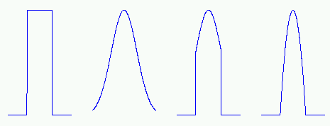Figure 3: The four neighborhood functions in SOM Toolbox: bubble, gaussian, cut gaussian and epanechicov (which is essentially max(0,1-x2)).

SOM algorithm

Size and shape

In the classical SOM, the number of neurons and their topological relations are fixed from the beginning. There are four issues which need to decided: the number of neurons, dimensions of the map grid, map lattice and shape.

The number of neurons should usually be selected as big as possible, with the neighborhood size controlling the smoothness and generalization of the mapping. The mapping does not considerably suffer even when the number of neurons exceeds the number of input vectors, if only the neighborhood size is selected appropriately. However, as the size of the map increases e.g. to tens of thousands of neurons the training phase becomes computationally impractically heavy for most applications.

In SOM Toolbox, the default number of neurons is 5 * sqrt(n) where n is the number of training samples. Note that the computational load increases quadratively with the number of map units. Therefore, don't take literally the "as big as possible" thing above. In our own research, the number of map units is usually between 100-600.

If possible, the shape of the map grid should correspond to the shape of the data manifold. Therefore, the use of toroid and cylinder shapes is only recommended if the data is known to be circular. For the default sheet shaped map, it is recommended that side length along one dimension is longer than the others, e.g. msize = [15 10], so that the map can orientate itself properly. One could possibly use the eigenvalues of the training data set as a guideline in setting the map grid side lengths.

The use of hexagonal lattice is usually recommended, because then all 6 neighbors of a neuron are at the same distance (as opposed to the 8 neighbors in a rectangular lattice). This way the maps become smoother and more pleasing to the eye. However, this is mostly a matter of taste.

In SOM Toolbox, the map grid sidelengths are determined by the ratio between eigenvalues of the training data. Also the compression of map units in case of hexagonal lattice (in vertical direction by a factor of sqrt(0.75)) is taken into account.

Initialization

Before the training, initial values are given to the prototype vectors. The SOM is very robust with respect to the initialization, but properly accomplished it allows the algorithm to converge faster to a good solution. Typically one of the three following initialization procedures is used:

• random initialization, where the weight vectors are initialized with small random values
• sample initialization, where the weight vectors are initialized with random samples drawn from the input data set
• linear initialization, where the weight vectors are initialized in an orderly fashion along the linear subspace spanned by the two principal eigenvectors of the input data set. The eigenvectors can be calculated using Gram-Schmidt procedure.

In SOM Toolbox, random and linear initializations have been implemented. Random initialization is done by taking randomly values from the d-dimensional cube defined by the minimum and maximum values of the variables. Linear initialization is done by selecting a mesh of points from the d-dimensional min-max cube of the training data. The axis of the mesh are the eigenvectors corresponding to the m greatest eigenvalues of the training data (m is the map grid dimension). Notice that the shape (e.g. cylinder) of the map is not taken into account in initialization: it is always assumed to be a sheet.

Training

In each training step, one sample vector x from the input data set is chosen randomly and a similarity measure is calculated between it and all the weight vectors of the map. The Best-Matching Unit (BMU), denoted as c, is the unit whose weight vector has the greatest similarity with the input sample x. The similarity is usually defined by means of a distance measure, typically Euclidian distance. Formally the BMU is defined as the neuron for which

||x - m_c|| = min_i{||x - m_i||},

where ||.|| is the distance measure.

After finding the BMU, the prototype vectors of the SOM are updated. The prototype vectors of the BMU and its topological neighbors are moved closer to the input vector in the input space. This adaptation procedure stretches the prototypes of the BMU and its topological neighbors towards the sample vector. This is illustrated in Figure 4. The SOM update rule for the weight vector of the unit i is:

m_i(t+1) = m_i + a(t) h_ci(r(t)) [x(t) - m_i(t)],

where t denotes time, a(t) is learning rate and h_ci(r(t)) the neighborhood kernel around the winner unit c, with neighborhood radius r(t).

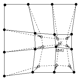Figure 4: Updating the best matching unit (BMU) and its neighbors towards the input sample marked with x. The solid and dashed lines correspond to situation before and after updating, respectively.

In SOM Toolbox, finding of BMU is slightly more complex, because the data samples may have missing components (NaNs), and each variable has an associated weighting factor, defined in field mask of map and training structs.
Missing components are handled by simply excluding them from the distance calculation (ie. it is assumed that their contribution to the distance ||x - m_i|| is zero). Because the same variable(s) is ignored in each distance calculation (over which the minimum is taken), this is a valid solution.
The weighting factor mask is primarily used in binary form for excluding certain variables from the BMU-finding process (1 for include, 0 for exclude). However, the mask can get any values, so it can be used for weighting variables according to their importance. With these changes, the distance measure becomes:

where K is the set of known (not missing) variables of sample vector x, x_k and m_k are kth components of the sample and prototype vectors and w_k is the kth mask value (mask(k)). Note though that the update rule does not change, so the weighting only affects finding of BMU.

Training parameters

The learning rate a(t) is a decreasing function of time between [0,1]. Two commonly used forms are a linear function and a function inversely proportional to time: a(t) = A / (t+B), where A and B are some suitably selected constants. Use of the latter function type ensures that all input samples have approximately equal influence on the training result.

In SOM Toolbox, there are three learning rate functions: linear, inverse-of-time, and a power series. These are illustrated in Figure 5. The power series is defined as

where a₀ is the initial learning rate, a_T the final learning rate, t is time and T the training length.

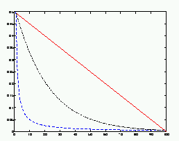Figure 5: The three learning rate functions in SOM Toolbox: linear (red), power series (black) and inverse-of-time (blue).

Also neighborhood radius typically decreases with time. Since large neighborhood radius makes the SOM more rigid, it is usually used in the beginning of training, and then it is gradually decreased to a suitable final radius. A suitable final radius is, for example, one. Notice that if neighborhood radius is set to zero r=0, the SOM algorithm reduces to k-means algorithm.

The total training time -- or, the number of samples presented to the SOM --- is an important consideration. The number of training steps should be at least 10 times the number of map units.

The training is usually performed in two phases. In the first phase, relatively large initial learning rate and neighborhood radius are used. In the second phase both learning rate and neighborhood radius are small right from the beginning. This procedure corresponds to first tuning the SOM approximately to the same space as the input data and then fine-tuning the map. If the linear initialization procedure is used the first training phase can be skipped.

In SOM Toolbox, the default is to train the map in two phases. The function som_train_struct.m defines the default training parameters. This is quite complex, but in principle, learning rate begins from 0.5 in the first phase, and from 0.05 in the second phase. Neighborhood radius starts from max(msize)/4 and goes down to one fourth of that (unless this would be less than 1). On second phase, neighborhood radius starts from where it stopped in first phase, and goes down to 1. The length of second phase is 4 times that of the first phase.

The training parameters are saved to a training struct, which can be found from the trainhist field of the map struct.

Batch training algorithm

An important variant of the basic SOM is the batch algorithm. In it, the whole training set is gone through at once and only after this the map is updated with the net effect of all the samples. Actually, the updating is done by simply replacing the prototype vector with a weighted average over the samples, where the weighting factors are the neighborhood function values.

where c(j) is the BMU of sample vector x_j, h_i,c(j) the neighborhood function (the weighting factor), and n is the number of sample vectors.

The default training algorithm in SOM Toolbox is this batch algorithm. This is because it is much faster to calculate in Matlab than the normal sequential algorithm, and the results are typically just as good or even better.

Variants

There are many variants to the basic SOM. One variantion theme is to use neuron-specific learning rates and neighborhood sizes. Another is to use adaptive or flexible neighborhood definitions or even growing map structures. The goal of these variations is to enable the SOM to follow better the topology of the underlying data set or to achieve better quantization results. A usual defect of these methods is that the visualization properties suffer or that the algorithm becomes computationally heavier. Another family of variations aims at making the SOM a better classifier.

Of the variants, SOM Toolbox has (at least) implementation of neural gas (neural_gas.m) and supervised SOM (som_supervised.m). There are also implementations of k-means (kmeans.m), kNN (knn.m) and LVQ (lvq1.m, lvq3.m).

<<< to Documentation main page