Kurtosis

The classical measure of nongaussianity is kurtosis or the fourth-order cumulant. The kurtosis of y is classically defined by

$$\:\mbox{kurt}(y)=E\{y^4\}-3(E\{y^2\})^2$$ (13)

Actually, since we assumed that y is of unit variance, the right-hand side simplifies to $E\{y^4\}-3$. This shows that kurtosis is simply a normalized version of the fourth moment $E\{y^4\}$. For a gaussian y, the fourth moment equals $3(E\{y^2\})^2$. Thus, kurtosis is zero for a gaussian random variable. For most (but not quite all) nongaussian random variables, kurtosis is nonzero.

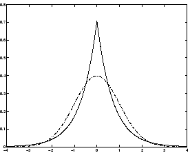
Kurtosis can be both positive or negative. Random variables that have a negative kurtosis are called subgaussian, and those with positive kurtosis are called supergaussian. In statistical literature, the corresponding expressions platykurtic and leptokurtic are also used. Supergaussian random variables have typically a ``spiky'' pdf with heavy tails, i.e. the pdf is relatively large at zero and at large values of the variable, while being small for intermediate values. A typical example is the Laplace distribution, whose pdf (normalized to unit variance) is given by

$$p(y)=\frac{1}{\sqrt{2}}\exp(\sqrt{2}\vert y\vert)$$ (14)

This pdf is illustrated in Fig. 8. Subgaussian random variables, on the other hand, have typically a ``flat'' pdf, which is rather constant near zero, and very small for larger values of the variable. A typical example is the uniform distibution in eq. (7).

  

Figure 8: The density function of the Laplace distribution, which is a typical supergaussian distribution. For comparison, the gaussian density is given by a dashed line. Both densities are normalized ot unit variance.

Typically nongaussianity is measured by the absolute value of kurtosis. The square of kurtosis can also be used. These are zero for a gaussian variable, and greater than zero for most nongaussian random variables. There are nongaussian random variables that have zero kurtosis, but they can be considered as very rare.

Kurtosis, or rather its absolute value, has been widely used as a measure of nongaussianity in ICA and related fields. The main reason is its simplicity, both computational and theoretical. Computationally, kurtosis can be estimated simply by using the fourth moment of the sample data. Theoretical analysis is simplified because of the following linearity property: If x₁ and x₂ are two independent random variables, it holds

$$\:\mbox{kurt}(x_1+x_2) = \:\mbox{kurt}(x_1) + \:\mbox{kurt}(x_2)$$ (15)

and

$$\:\mbox{kurt}(\alpha x_1) = \alpha^4 \:\mbox{kurt}(x_1)$$ (16)

where $\alpha$ is a scalar. These properties can be easily proven using the definition.

To illustrate in a simple example what the optimization landscape for kurtosis looks like, and how independent components could be found by kurtosis minimization or maximization, let us look at a 2-dimensional model ${\bf x}={\bf A}{\bf s}$. Assume that the independent components s₁, s₂have kurtosis values $\:\mbox{kurt}(s_1), \:\mbox{kurt}(s_2)$, respectively, both different from zero. Remember that we assumed that they have unit variances. We seek for one of the independent components as $y = {\bf w}^T{\bf x}$.

Let us again make the transformation ${\bf z}={\bf A}^T{\bf w}$. Then we have $y = {\bf w}^T{\bf x}={\bf w}^T{\bf A}{\bf s}={\bf z}^T{\bf s}= z_1s_1 + z_2s_2$. Now, based on the additive property of kurtosis, we have $\:\mbox{kurt}(y) = \:\mbox{kurt}(z_1s_1) + \:\mbox{kurt}(z_2s_2) = z_1^4 \:\mbox{kurt}(s_1) + z_2^4 \:\mbox{kurt}(s_2)$. On the other hand, we made the constraint that the variance of y is equal to 1, based on the same assumption concerning s₁, s₂. This implies a constraint on ${\bf z}$: $E\{y^2\} = z_1^2 + z_2^2 = 1$. Geometrically, this means that vector ${\bf z}$ is constrained to the unit circle on the 2-dimensional plane. The optimization problem is now: what are the maxima of the function $\vert\:\mbox{kurt}(y)\vert = \vert z_1^4 \:\mbox{kurt}(s_1) + z_2^4 \:\mbox{kurt}(s_2)\vert$ on the unit circle? For simplicity, you may consider that the kurtosis are of the same sign, in which case it absolute value operators can be omitted. The graph of this function is the "optimization landscape" for the problem.

It is not hard to show [9] that the maxima are at the points when exactly one of the elements of vector ${\bf z}$ is zero and the other nonzero; because of the unit circle constraint, the nonzero element must be equal to 1 or -1. But these points are exactly the ones when yequals one of the independent components $\pm s_i$, and the problem has been solved.

In practice we would start from some weight vector ${\bf w}$, compute the direction in which the kurtosis of $y = {\bf w}^T{\bf x}$ is growing most strongly (if kurtosis is positive) or decreasing most strongly (if kurtosis is negative) based on the available sample ${\bf x}(1), ... , {\bf x}(T)$ of mixture vector ${\bf x}$, and use a gradient method or one of their extensions for finding a new vector ${\bf w}$. The example can be generalized to arbitrary dimensions, showing that kurtosis can theoretically be used as an optimization criterion for the ICA problem.

However, kurtosis has also some drawbacks in practice, when its value has to be estimated from a measured sample. The main problem is that kurtosis can be very sensitive to outliers [16]. Its value may depend on only a few observations in the tails of the distribution, which may be erroneous or irrelevant observations. In other words, kurtosis is not a robust measure of nongaussianity.

Thus, other measures of nongaussianity might be better than kurtosis in some situations. Below we shall consider negentropy whose properties are rather opposite to those of kurtosis, and finally introduce approximations of negentropy that more or less combine the good properties of both measures.