Blind deconvolution

Blind deconvolution¹ is different from the other techniques discussed in this Section in the sense that (in the very simplest case) were are dealing with one-dimensional time signals (or time series) instead of multidimensional data, though blind deconvolution can also be extended to the multidimensional case. Blind deconvolution is an important research topic with a vast literature. We shall here describe only a special case of the problem that is closely connected to ours.

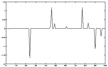
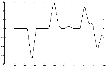
In blind deconvolution, a convolved version x(t) of a scalar signal s(t) is observed, without knowing the signal s(t) or the convolution kernel [126,42,54,53,92,129,130,148]. The problem is then to find a separating filter h so that s(t)=h(t)*x(t). An illustration can be found in Fig. 3.

  

Figure 3: An illustration of blind deconvolution. The original signal is depicted on the left. On the right, a convolved version of the signal is shown. The problem is then to recover the signal on the left, observing only the signal on the right.

The equalizer h(t) is assumed to be a FIR filter of sufficient length, so that the truncation effects can be ignored. A special case of blind deconvolution that is especially interesting in our context is the case where it is assumed that the values of the signal s(t) at two different points of time are statistically independent. Under certain assumptions, this problem can be solved by simply whitening the signal x(t). However, to solve the problem in full generality, one must assume that the signal s(t) is non-Gaussian, and use higher-order information [53,129]. Thus the techniques used for solving this (special case of the) problem are very similar to the techniques used in other higher-order methods discussed in this Section.